Just Enough Algebra

Lung cancer, chronic bronchitis, bad breath, stains on your clothes, and the expense. These are just a few of the consequences of smoking cigarettes. With what we know now about the dangers of smoking, are people smoking more or less than they were ten years ago, fifty years ago, or even one hundred years ago?

Reality is, we don’t have information on each individual person’s smoking rate, so we can’t answer this question exactly. We do have information on the total number of cigarettes sold each year. So maybe we should look at that total. Uh oh, that isn’t going to work. There are way more people now than there were fifty or a hundred years ago. So, even if the same percentage of people smoke, and even if they each smoke the same amount as their predecessors did, we would have a much bigger number of cigarettes smoked now just because there are more people now.

Turns out a reasonable measure is to compare the number of cigarettes smoked per year per person. By taking into account the number of people we will be able to see whether people are smoking more or less, on average. That’s what we want.

The table showing the smoking rate for select years. The smoking rate is the average cigarettes per year per person (adults).

We can tell a lot of information from this table. For example, what was the smoking rate in 1965, and how does that compare to 2006? The answers appears in the table, a whopping 4,258 cigarettes per person in 1965 and 1,619 cigarettes per person in 2006.

When did the consumption first pass 3,000? That answer does not appear in the table, but we can use the information in the table to make a good guess. In 1940, there were an average of 1,976 cigarettes per person per year and by 1950, there were 3,552. Somewhere between 1940 and 1950 the number first climbed above 3,000. More specifically, the number we’re looking for (3,000) is a lot closer to the 1950 figure (3,552) than to the 1940 figure (1,976). So, it would be reasonable to guess close to 1950. I’d say 1947. Of course, you might guess 1946 or 1948, or even 1949 and those would be good guesses too.

When did the consumption drop below 3,000 again? This answer also does not appear in the table, but falls somewhere between 1975 when consumption was 4,122 and 1990 when consumption was 2,834. Here I’d guess just before 1990, say in 1989.

Notice where the variable names are listed in the table. In a horizontal format like this table, the independent variable (\(Y\)) is in the top row, with the dependent variable (\(S\)) is in the bottom row. If you want to write your table in a vertical format, that’s okay too. Just put the independent variable in the left column, with the dependent variable in the right column. It might help to remember that the independent variable goes first (either top or left) and the dependent variable follows (either bottom or right).

Where the variables go in a table is not something you can figure out. It’s a convention - a custom, practice, or standard used within the mathematical community. Though based on reason, it often involves some arbitrary choice, which is why we can’t figure it out. So, whenever some practice is introduced to you as a “convention,” you need to memorize it.

Tables are useful because they contain specific numbers, but it can be difficult to guess or see general trends. For that, a picture is worth a thousand words - or numbers, in this case. By “picture” we mean a graph of the function.

Throughout this text, we draw graphs by hand. On graph paper. Seriously. You might wonder why we do that when graphing calculators, spreadsheet programs, graphing “apps,” or computer algebra systems all can draw graphs for us. The answer is we want to understand graphs better, and I promise that drawing them by hand will help you do that. (Different instructors have different opinions on the importance of graphing by hand, so be sure to ask your instructor what you are expected to do. Even if you’re allowed to use some type of graphing technology, I strongly encourage you to practice drawing graphs by hand as well.)

There is a standard set-up for a graph.

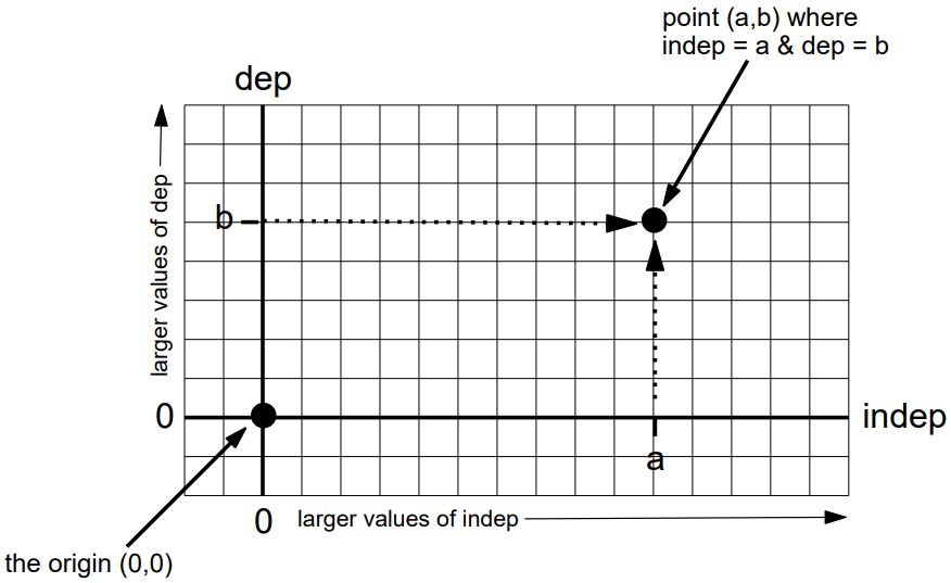
The graph is based on a horizontal line and vertical line, called the axes.

Aside

Where they cross is a point called the origin. It represents where each variable is 0. By convention, the independent variable is measured along the horizontal axis, with larger values progressing to the right of the origin, and negatives to the left. Similarly, the dependent variable is measured along the vertical axis, with larger values progressing up from the origin, and negatives down. Each gridline counts the same number, called the scale, but the scale for the vertical may be different from the scale for the horizontal. Each pair of values of the independent and dependent variable from our table correspond to a point on our graph.

In the graph of smoking rates, the independent variable is \(Y\text{,}\) the year, so that goes on the horizontal axis for our graph. Our dependent variable is \(S\text{,}\) the smoking rate, so that goes on the vertical axis. For the scale, it works nicely to count by 10s for years and count by 500s for the smoking rate.

There’s a certain amount of guess and check involved in figuring out a good scale for each axis. As a general rule of thumb we would like the graph to be as large as possible so we can see all of its features clearly. But, not so big that it runs off the graph paper. What matters is that the gridlines are evenly scaled and that they can handle large enough numbers. Speaking of which, it’s a good idea to leave a little room to extend the graph a little further than the information we have in the table, in case we get curious about values beyond what we have already.

With realistic numbers it’s normal to have numbers in the table that are not exactly where the gridlines are. It is very helpful to count by round numbers (2s, 5s, 10s, etc.) because it makes guessing in between easier. Easier for you drawing the graph. Easier for someone reading your graph.

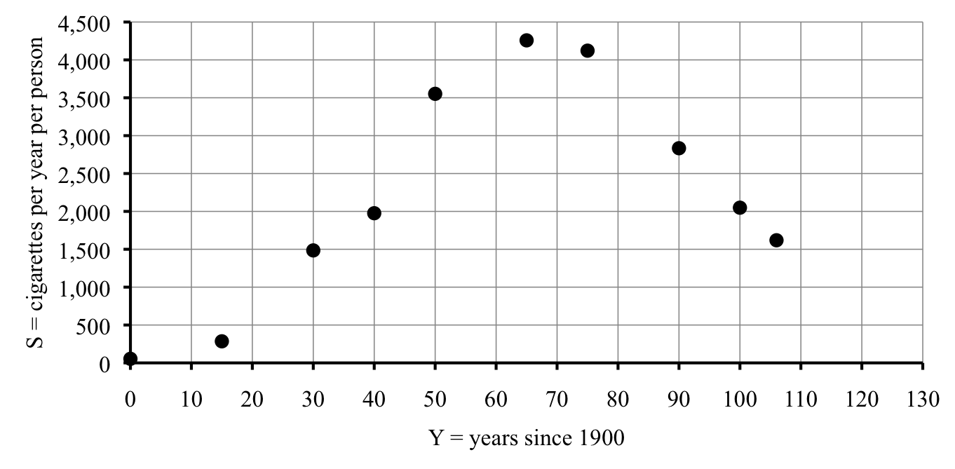
To plot each point, we start at the origin and move right to that \(Y\)-value, and then up to that \(S\)-value. When a value doesn’t land exactly on a grid mark, we have to guess in between. For example, in 1900, \(Y=0\) so we don’t move right at all, just up to \(S=54\text{.}\) The first labeled gridline on our graph is 500. Where’s 54? It’s between 0 and 500, very close to 0. Our point is just a tiny bit above the origin. In 1915 we have \(Y=15\text{.}\) Our labeled gridlines are for 10 and 20, so 15 must land halfway in between. The smoking rate is 285, which is around halfway between 0 and 500. Etc.

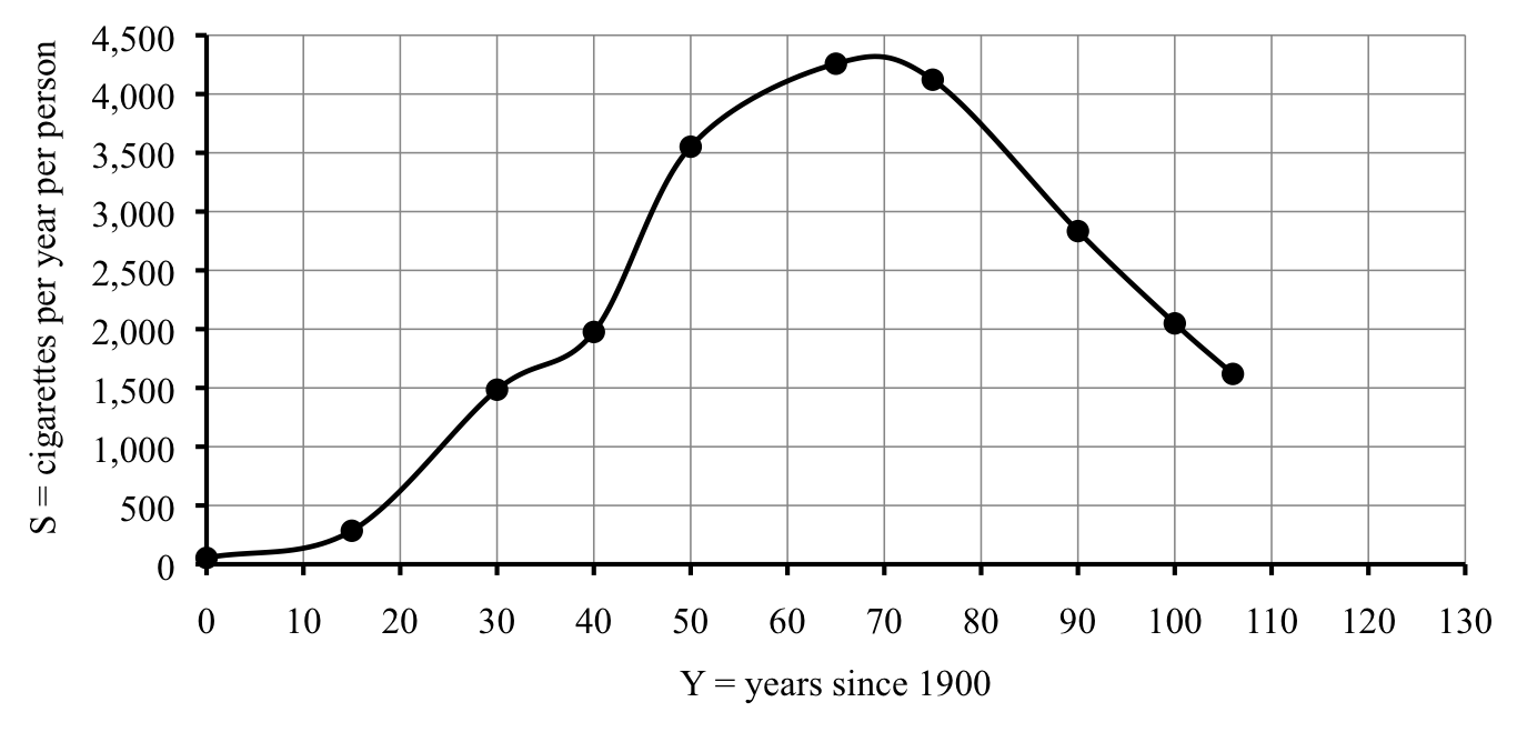
What we have so far is a scatter plot of points. Can you see why it’s called that? Anyway, our whole goal here was to be able to understand smoking rates better by having a graph. You may already begin to see a curve suggested by the points. Time to draw it in. I don’t mean drawing a line between each pair of points, like you do in the children’s game “connect the dots.” That isn’t quite right. It was probably more of a continuous trend and so the graph should be smoother.

When we draw in this smooth curve for the graph, what we are really doing is making a whole lot of guesses all at once. For example, from the table we guessed that the smoking rate passed 3,000 in around 1947, and dropped back to that level in around 1989. What does the graph show? If we look where the horizontal gridline for 3,000 crosses our graph, it crosses in two places. First, between the vertical gridlines for 40 and 50, and perhaps slightly closer to 50. I’d say \(Y \approx 47\text{,}\) in the year 1947. Sure. The second time is between the gridlines for 80 and 90, much closer to 90. Looks like \(Y \approx 88\text{,}\) in the year 1988. We guessed 1989. Close enough.

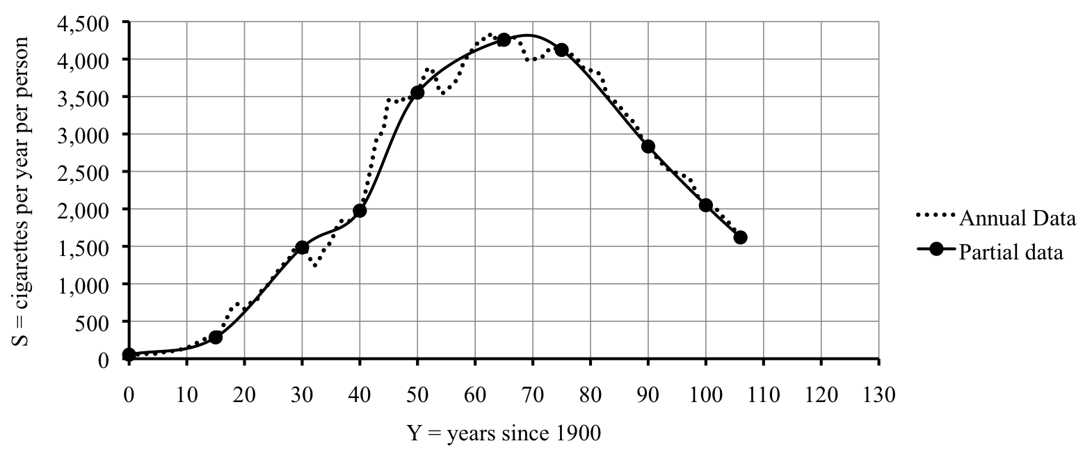
Don’t forget that when we drew in that curve it was really just a guess. We’re sure about the points we plotted, but we’re only guessing about where to draw the curve in. That means we’re not sure about the other points. If we knew a lot more points we could have a more accurate graph.

Turns out more data is available from the CDC. The full table of data from the CDC shows that consumption first topped 3,000 as early as 1944. Here’s an example where the history tells you more than the mathematics as cigarette consumption rose sharply during World War II. Our guess about 1988 or 1989 was spot on. Look at how the graph from the full data (the dotted line) compares to our guess.